Introduction
Ray tracing is a simple yet very powerful technique for doing photo-realistic rendering. It is physics based, and is one of the backbone technologies in the filming and gaming industry.
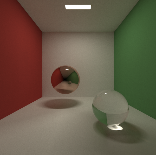
In this series of articles, we are going to write a ray tracer that renders a Cornell Box scene (well, not an authentic one). Eventually, you should be able to get something like this on your screen:
Background
I quoted Python in the title because I lied. No, we are not using Python, but a sibling language called Taichi.
Taichi (太极) is a programming language designed for high-performance computer graphics. It is deeply embedded in Python3, and its just-in-time compiler offloads the compute-intensive tasks to multi-core CPUs and massively parallel GPUs.
In another word, Taichi offers the simplicity of Python and the performace of the hardware, the best of both.
Before you shake your head and mumble “I don’t want to learn a new language just for that”, don’t worry. I assure you that there is nothing new about the language itself. You will be writing native Python, and can view Taichi just as a powerful library. In fact, here’s how you’d want to install it (Note that Taichi is only available since Python 3.6+):
python3 -m pip install taichi
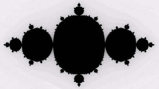
And here’s a peek of it:
import taichi as ti

ti.init(arch=ti.gpu)
n = 320
pixels = ti.var(dt=ti.f32, shape=(n * 2, n))

@ti.func
def complex_sqr(z):
    return ti.Vector([z[0]**2 - z[1]**2, z[1] * z[0] * 2])

@ti.kernel
def paint(t: ti.f32):
    for i, j in pixels:  # Parallized over all pixels
        c = ti.Vector([-0.8, ti.cos(t) * 0.2])
        z = ti.Vector([float(i) / n - 1, float(j) / n - 0.5]) * 2
        iterations = 0
        while z.norm() < 20 and iterations < 50:
            z = complex_sqr(z) + c
            iterations += 1
        pixels[i, j] = 1 - iterations * 0.02

gui = ti.GUI("Julia Set", res=(n * 2, n))
for i in range(1000000):
    paint(i * 0.03)
    gui.set_image(pixels)
    gui.show()
which renders a nice Julia Set:
Most of the code should look familiar (from the Python’s perspective, not the algorithm it implements), except for those seemingly innocenet decorators like @ti.func and @ti.kernel. In fact, they are what Taichi is all about. There is also some boilerplate code you need to write, and we will jump into all that in just a moment.
One more thing I should mention before we start. Here is a list of some awesome references I’ve found for learning ray tracers and computer graphics (CG).
- Ray Tracing in One Weekend: The content on this site is such a delight to read. It comes in three brochures, but if you only want to code something fancy, then the first one is more than enough to get things going. In fact, I should give 90% of the credits to the author 1, because most of the ray tracing theory and implementation that I’m covering here is just an unashamedly copy of the first article. One possible bummer is that it is taught in C++, which is also why I was originally motivated to write this post.
- Phyisicall Based Rendering: From Theory To Implementation: For anyone who is seriously considering to work on the CG field, this book is a must read. However, it is way too advanced for the purpose of this tutorial. We will borrow some ideas from it in the third post. For now, you can safely ignore it.
- Real Time Rendering: In my opinion, this book is more approachable than the previous one. While it focuses on the real time side (the other end being photorealism), the topics from Chapter 9 to 11 still offer a decent summary of the ray casting and ray tracing techniques.
- MIT 6.837 Computer Graphics: This course was where I started to learn about CG. It is not only about ray tracing, but covers a broader range of topics in CG.
- UCSB CS 180: Introduction to Computer Graphics: I haven’t taken this course, but the materials look more relevant and modernized compared to MIT 6.837. 该课程还有中文版,详见:Games 101: 现代计算机图形学入门
- Kajiya, J.T., 1986, August. The rendering equation: The paper laying the foundation of ray tracing.
- Veach, E. and Guibas, L.J., 1995, September. Optimally combining sampling techniques for Monte Carlo rendering: This paper uses multiple importance sampling (MIS) to improve the rendering quality. It has some advanced, but still managable, statistics behind. We will be covering this in the third post of the series.
Enough said, let’s get started!
Hello Taichi
Before we can do anything, we need to be able to draw pixels on the screen. A screen of pixels is nothing more than a 2D array of RGB values, i.e. each element in the array is a tuple of three floating points. Note that the RGB component in Taichi is between 0.0 and 1.0, not 0 to 0xff.
import taichi as ti

sz = 800
res = (sz, sz)

ti.init(arch=ti.gpu)
color_buffer = ti.Vector(3, dt=ti.f32, shape=res)
If you’ve used numpy before, it may already look familiar to you of how color_buffer is defined. Concretely, we have instantiated a 2-D Taichi tensor of shape=(800, 800), and assigned it to color_buffer. Each element in color_buffer is a ti.Vector containing three 32-bit floating point numbers (ti.f32).
I should also expand a bit more on ti.init(arch=ti.gpu). Obviously, it does some initialization. At a minimum, you need to tell Taichi on which hardware architecture you want the program to run. There are two options here: ti.gpu or ti.x64, for targeting at GPU and CPU, respectively.
Because Taichi is designed for computer graphics (or any sort of massively parallelizable computations for that matter), it is always preferrable to target at GPU first. Currently, Taichi supports these GPU platforms, and will choose the available one automatically:
- CUDA
- Apple Metal
- OpenGL, with compute shader support
However, when none of these is avaialble, Taichi will fallback to the CPU architecture. But even in that case, Taichi will still parallelize your computational tasks, just via a CPU thread pool.
Here comes the beauty of Taichi: Once you do get access to another device with the listed GPUs support, your Taichi program will be ported to it seamlessly, and immediately enjoy the benefits of massive parallelization powered by GPU.
Let’s get back to rendering. We need to assign some color to it and display the array on the screen.
@ti.kernel
def render():
    for u, v in color_buffer:
        color_buffer[u, v] = ti.Vector([0.678, 0.063, v / sz])


gui = ti.GUI('Cornell Box', res)
for i in range(50000):
    render()
    img = color_buffer.to_numpy(as_vector=True)
    gui.set_image(img)
    gui.show()

input("Press any key to quit")
Here, we have encountered our first Taichi kernel, render(). It is decorated by @ti.kernel. When render() is called for the first time, Taichi will JIT compile the decorated Python function to Taichi IR, and finally to platform specific code (LLVM for x86/64 or CUDA, Metal Shader Language, or GLSL). None of these implementation details matters from the users’ perspective, so don’t worry if the workflow doesn’t immediately make sense. What you only need to remember is that, while your Taichi kernel is written in the Python syntax, internally the code is completely taken over and optimized by the Taichi compiler and runtime.
What’s special about the Taichi kernel is that, during the kernel compilation, it automatically parallelizes the top-level for loop. So inside render():
    for u, v in color_buffer:
        color_buffer[u, v] = ti.Vector([0.678, 0.063, v / sz])
You can think of each (u, v) coordinate as being executed on its own thread 2. As a result, what is expected to run sequentially in Python will actually run in parallel.
This kind of for loop is called struct-for loops. It is an idiomatic way to loop over a tensor in Taichi. (u, v) will loop over the 2-D mesh grid as defined by the shape of color_buffer, i.e. (0, 0), (0, 1), ..., (0, 799), (1, 0), ..., (799, 799).
Now that we have covered the essential part, the rest should be relatively easy to explain.
gui = ti.GUI('Cornell Box', res)
This just creates a drawable GUI window titled Cornell Box, with resolution 800x800. Taichi comes with a tiny GUI system that is portable on all the major OSes, including Windows, Linux and Mac.
for i in range(50000):
    render()
    img = color_buffer.to_numpy(as_vector=True)
    gui.set_image(img)
    gui.show()
Calling a Taichi kernel is no different from a regular Python function. For the first call, Taichi JIT compiles render() to the low-level machine code, and runs it directly on GPU/CPU. Subsequent calls will skip the compilation step, since the compiled kernel will be cached by the Taichi runtime.
Once the execution completes, we need to transfer the data back. Here comes another nice thing: Taichi has already provided a few helper methods so that it can easily interact with numpy and pytorch. In our case, the Taichi tensor is converted into a numpy array called img, which is then passed into gui to set the color of each pixel. At last, we call gui.show() to update the window. Although for i in range(50000): might seem redundant, we will soon need it when doing ray tracing.
Let’s name the file box.py and run it with python3 box.py. If you see the window below, congratulations! You have successfully run your first Taichi program.
Ray Tracing in 10 Minutes
Before any more coding, we need some preliminary knowledge on how the ray tracing algorithm works. If you are already an expert on this topic, feel free to jump to the next section. Otherwise, I will give a brief introduction of the algorithm. In the meantime, I’d still recommend you to read on Ray Tracing in One Weekend. There is no way I could do a better job than that article.
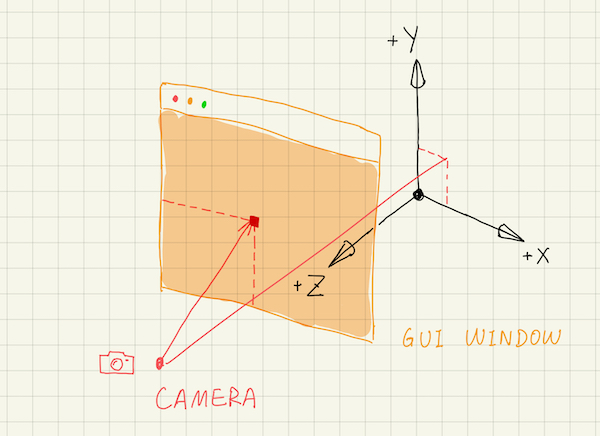
We need a coordinate space to precisely describe the scene. We will be using a right-hand coordinate frame. That is, the plane of your screen defines the x and y axes, where the x axis points to the right, and the y axis upward. The z axis points outwards from the screen towards you. This coordinate frame is referred to as the world space.
If you think of the GUI as a window in the world space that sits in front of the scene, the ray tracer will send a ray from a fixed position through every pixel on that window. That fixed position is where the (virtual) camera is located in the world space. The color of the pixel is then that of the closest object hit by the ray.
We call the process sampling for sending a ray through a pixel and tracing it inside the scene. It is usually not enough to sample the pixels just once, as the output image will be very noisy. A simple mitigation (with solid statistics foundation!) is to sample multiple times, then sum up the color to compute the mean. Of course, it would be meaningless if all the samplings trace exactly the same path. We shall see shortly that randomness will be added to the sampling process at multiple places. (I mean, why bother calling it sampling if there was no randomness involved?)
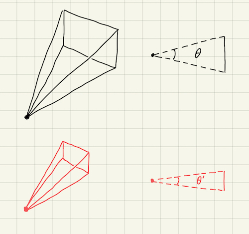
If you connect the camera position with the four corners of the window, you will get a frustum. Only those objects located within this frustum volume will be rendered on the screen. One problem is that, we only know the width to height ratio (the aspect ratio) of the cross section rectangle, which is the same as that of the GUI window, but not its area. Consequently, we don’t know the frustum’s volume.
One solution is to define the coordinates of the window’s four corners in the world space. However, there is a simpler approach. We add a new paramter to the camera system, called the field of view (fov). Informally speaking, this measures how wide the frustum opens up vertically. The figure below shows that, although the cross section rectangles of the two frustums have the same aspect ratio, because the top frustum has a larger fov (\(\theta \gt \theta^\prime\)), it can cover a larger chunk of the scene.
We can ask a few questions about the ray tracing technique now:
- How to describe a ray from a mathematics point of view?
- How to find the closest object the ray intersects? Moreover, not only do we want to know the object, but also the precise intersection point on that object.
- How to compute the color of the pixel?
A ray can be defined by its origin, \(\boldsymbol{o}\), and its direction \(\boldsymbol{d}\). (We use a bold \(\boldsymbol{x}\) to denote that this is a 3-D vector, i.e. \(\boldsymbol{x} \in \mathbb{R}^3\).) Given these two parameters, any point along the ray can be uniquely identified by a positive real number \(t\): \[\boldsymbol{r}(t) = \boldsymbol{o} + \boldsymbol{d} \cdot t\]
A point that is closer to the camera, or more generally, the ray origin \(\boldsymbol{o}\), will have a smaller \(t\).
To find out the closest hitting point, we start with \(t = +\infty\), iterate over every object in the scene and check for ray-object intersection. In code, t is initialized to an extremetely large number, e.g. 1e10. If the ray does hit an object, \(t\) is updated, but only if the intersection results in a smaller \(t\). How exactly the intersection point is computed, if there is any, depends on the gemoetry of that object. Fortunately, it is relatively easy to write out the intersection equations for all the geometris we will be using in this example. Concretely, there are three types of geometries: plane, axis aligned rectangle and sphere. The difference between a plane and a rectangle is that the later is bounded.
For the third question, it is really about how to compute the color of a point on a given object, with a given ray. To be able to answer this, we need to introduce another concept, material.
Material is the key to determine an object’s appearance, including its color, its textural feeling, etc. Is it matte? Is it metallic? Is it transparent? … As the ray intersects with an object, we will also record the material associated with that object.
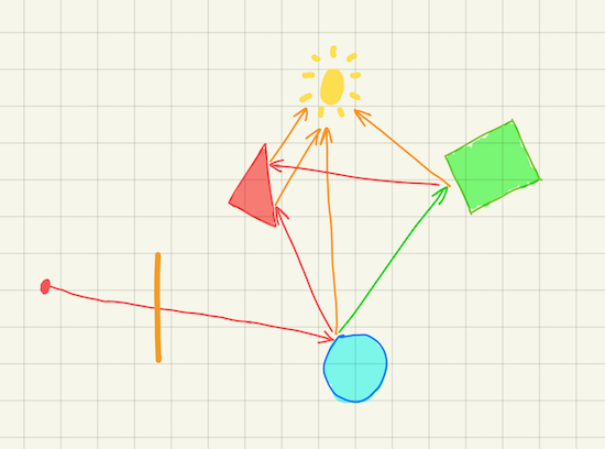
Let me take a step back from the materials, and give a broad overview of how the ray is traced.
Once the ray from the camera hits an object, we have two choices here. The first option is to compute the color using the light sources information, and end the sampling here. This is effectively the local illumination shading model, because it only takes into account the interaction between the object and the light sources.
Alternatively, we record the color and the material information, then shoot a new ray from the intersection point, and continue the sampling process. The direction of this new ray depends on the hitting material, which could be either probablistic or deterministic. When the new ray hits another object, record the color ‘n material, shoot a third ray, and so on so forth. To prevent it from running forever, we can put a cap on how many times the ray can bounce, called the maximum ray-tracing depth.
The accumulated color information is called the throughput. In the beginning, it is set to 1.0 for all its RGB components. Each time the ray hits a regular object (i.e. not a light source), throughput is multiplied with the color of that point. In the end, throughput is attenuated by the colors of all the intersected points along the path: \[\begin{aligned} throughput = \prod_{i=1}^n color_{i} \end{aligned}\]
If the ray manages to hit a light source before reaching the maximum depth, the sampled color is the product of throughput and the light source color. Otherwise, the entire path being traced was not lit, and the sampled color is just pure black.
This shading model is called global illumination, and is performed recursively (which can be turned into an iterative process, thankfully). The color sampled for a pixel therefore accounts for the illumnination from both the light sources directly, and the indirect reflection of the lights through other objects that are not emissive by themselves. As a result, we can get a much more realistic image with very vivid effects, such as soft shadows and caustics.
This completes the ray tracing algorithm in its entirety. Hopefully, by now you would recognize its conciseness, and be amazed at its efficacy. However, the devil is in the detail. We now turn back to the materials to understand how to choose a new ray direction.
There are two materials used in this post: lambertian and emissive.
Lambertian is probably the simplest reflective material that models perfect diffusion. It scatters the incident ray to all the direction above the hitting surface with equal probability. Lambertian material doesn’t emit lights on its own, but its does have an intrinsic color.
Emissive material, as its name indicates, emits light. An object with such a material is called a light source, and has the capability of affecting the appearance of other objects. Emissive material is actually simpler than lambertian, because it is not reflective. When the ray hits a light source, we can terminate the sampling earlier without spawning a new ray. This might not be physically sound, but it simplifies the ray tracing algorithm while the result still looks reasonably correct, since the light color is usually the dominant factor.
There are other reflective materials, e.g. the glass sphere on the right side of the cover image. However, we will address these more advanced materials in a later post.
Think in the Box
We need some helpers from math and numpy, go import them:
# import taichi as ti
import numpy as np
import math
We also need to define a few constants:
# ...
# res = (sz, sz)
aspect_ratio = res[0] / res[1]

eps = 1e-4
inf = 1e10
fov = 0.8
max_ray_depth = 10

mat_none = 0
mat_lambertian = 1
mat_light = 2

camera_pos = ti.Vector([0.0, 0.6, 3.0])
light_color = ti.Vector([0.9, 0.85, 0.7])

# ti.init(arch=ti.gpu)
# ...
eps: A tiny fraction to help resolve the numerical errors in certain cases.max_ray_depth: The maxinum depth a ray can trace inside the scene.mat_*: These are the material enums.mat_noneis a special mark to indicate that the ray hits nothing.
Other constants should be self explanatory.
Since we are observing within a box, we need to construct a total of five sides of the box. A side can be represented using an infinite plane. How do we describe that mathematically?
If we are given a point on an infinite plane, \(\boldsymbol{x}\), and its normal, \(\boldsymbol{n}\), then for any point \(\boldsymbol{p}\) on that plane, we know that \(\boldsymbol{p} - \boldsymbol{x}\) must be perpendicular to \(\boldsymbol{n}\): \[\begin{aligned} (\boldsymbol{p} - \boldsymbol{x}) \cdot \boldsymbol{n} = \boldsymbol{0} \end{aligned}\]
Since \(\boldsymbol{p}\) is also along the ray, i.e. \(\boldsymbol{p}(t) = \boldsymbol{o} + \boldsymbol{d}\cdot t\), we have: \[\begin{aligned} (\boldsymbol{p}(t) - \boldsymbol{x}) \cdot \boldsymbol{n} = \boldsymbol{0} \\ (\boldsymbol{o} + \boldsymbol{d} \cdot t - \boldsymbol{x}) \cdot \boldsymbol{n} = \boldsymbol{0} \\ (\boldsymbol{d} \cdot \boldsymbol{n}) \cdot t = (\boldsymbol{x} - \boldsymbol{o}) \cdot \boldsymbol{n} \\ t = \frac{(\boldsymbol{x} - \boldsymbol{o}) \cdot \boldsymbol{n}}{\boldsymbol{d} \cdot \boldsymbol{n}} \end{aligned}\]
We can now define a function to check if a ray would intersect with a given plane:
@ti.func
def ray_plane_intersect(pos, d, pt_on_plane, norm):
    t = inf
    denom = ti.dot(d, norm)
    if abs(denom) > eps:
        t = ti.dot((pt_on_plane - pos), norm) / denom
    return t
Here, we have seen a new Taichi decorator, @ti.func. This one is handled in a similar way as @ti.kernel is, in that the decorated function is compiled to native machine code, and executed without the Python interpreter. Because of this, functions decorated with @ti.func can only be called from another function that is decorated by either @ti.kernel or @ti.func, but not from the Python scope.
Most of the procedure inside ray_plane_intersect() is a direct translation of the equations above. Note that there is a possibility where the ray direction \(\boldsymbol{d}\) is in parallel with the plane. In another word, it is perpendicular to the plane normal \(\boldsymbol{n}\). We compute \(t\) only if that is not the case, i.e. \(\boldsymbol{d} \cdot \boldsymbol{n} \ge \epsilon\).
In the previous section, we have explained that when shooting a ray, we need to find out the closest point it hits. Let’s define such a function:
@ti.func
def intersect_scene(ray_o, ray_d):
closest, normal = inf, ti.Vector.zero(ti.f32, 3)
color, mat = ti.Vector.zero(ti.f32, 3), mat_none
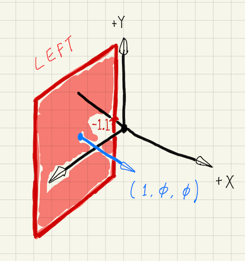
# left
pnorm = ti.Vector([1.0, 0.0, 0.0])
cur_dist = ray_plane_intersect(ray_o, ray_d, ti.Vector([-1.1, 0.0, 0.0]),
pnorm)
if 0 < cur_dist < closest:
closest = cur_dist
normal = pnorm
color, mat = ti.Vector([0.65, 0.05, 0.05]), mat_lambertian
return closest, normal, color, mat
closest and normal are used to store the final \(t\) and the normal of the hit surface, respectively. color and mat store the color and the material enum of the hit surface. If nothing is hit, these value will not be modified. One restriction that I should point out: Currently, Taichi function doesn’t support multi-return yet. So you will have to pre-define all the variables that will be returned at the top. A bit cumbersome, but not a big deal.
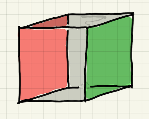
As a start, we have only defined the left side plane of the box. This plane passes point [-1.1, 0.0, 0.0] and has a normal of [1.0, 0.0, 0.0]. In another word, this is a \(yz\) plane pointing to the \(+x\) direction, and intersecting the \(x\) axis at -1.1. Its material is lambertian (mat_lambertian), with a red color (RGB = [0.65, 0.05, 0.05]).
We can add the right, top, bottom and far side planes in a similar way. Below shows the complete function definition:
@ti.func
def intersect_scene(ray_o, ray_d):
    closest, normal = inf, ti.Vector.zero(ti.f32, 3)
    color, mat = ti.Vector.zero(ti.f32, 3), mat_none

    # left
    pnorm = ti.Vector([1.0, 0.0, 0.0])
    cur_dist = ray_plane_intersect(ray_o, ray_d, ti.Vector([-1.1, 0.0, 0.0]),
                                   pnorm)
    if 0 < cur_dist < closest:
        closest = cur_dist
        normal = pnorm
        color, mat = ti.Vector([0.65, 0.05, 0.05]), mat_lambertian
    # right
    pnorm = ti.Vector([-1.0, 0.0, 0.0])
    cur_dist = ray_plane_intersect(ray_o, ray_d, ti.Vector([1.1, 0.0, 0.0]),
                                   pnorm)
    if 0 < cur_dist < closest:
        closest = cur_dist
        normal = pnorm
        color, mat = ti.Vector([0.12, 0.45, 0.15]), mat_lambertian
    # bottom
    gray = ti.Vector([0.93, 0.93, 0.93])
    pnorm = ti.Vector([0.0, 1.0, 0.0])
    cur_dist = ray_plane_intersect(ray_o, ray_d, ti.Vector([0.0, 0.0, 0.0]),
                                   pnorm)
    if 0 < cur_dist < closest:
        closest = cur_dist
        normal = pnorm
        color, mat = gray, mat_lambertian
    # top
    pnorm = ti.Vector([0.0, -1.0, 0.0])
    cur_dist = ray_plane_intersect(ray_o, ray_d, ti.Vector([0.0, 2.0, 0.0]),
                                   pnorm)
    if 0 < cur_dist < closest:
        closest = cur_dist
        normal = pnorm
        color, mat = gray, mat_lambertian
    # far
    pnorm = ti.Vector([0.0, 0.0, 1.0])
    cur_dist = ray_plane_intersect(ray_o, ray_d, ti.Vector([0.0, 0.0, 0.0]),
                                   pnorm)
    if 0 < cur_dist < closest:
        closest = cur_dist
        normal = pnorm
        color, mat = gray, mat_lambertian

    return closest, normal, color, mat
The properties of each side are summarized in the following table.
| side | axis-aligned plane | normal | intersecting axis | color |
|---|---|---|---|---|
| left | yz | +x | x = -1.1 | [0.65, 0.05, 0.05] (Red) |
| right | yz | -x | x = 1.1 | [0.12, 0.45, 0.15] (Green) |
| bottom | xz | +y | y = 0.0 | [0.93, 0.93, 0.93] (Gray) |
| top | xz | -y | y = 2.0 | [0.93, 0.93, 0.93] (Gray) |
| far | xy | +z | z = 0.0 | [0.93, 0.93, 0.93] (Gray) |
Oh Shoot
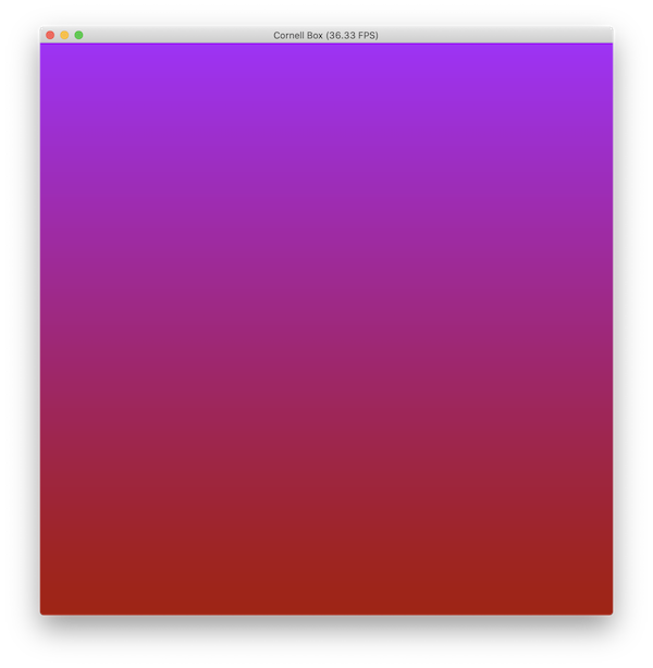
We have done a great amount of work now, yet the main render() kernel remains unchanged. If you run box.py now, it still renders that mundane gradient color view.
“Oh shoot! How am I supposed to see my hard work?”
Exactly, let’s shoot some rays into the scene :)
@ti.kernel
def render():
    for u, v in color_buffer:
        ray_pos = camera_pos
        ray_dir = ti.Vector([
            (2 * fov * (u + ti.random()) / res[1] - fov * aspect_ratio),
            (2 * fov * (v + ti.random()) / res[1] - fov),
            -1.0,
        ])
        ray_dir = ti.normalized(ray_dir)
The first ray always starts at the camera position. The ray direction deserves more attention. Take a look at the y component first:
(2 * fov * (v + ti.random()) / res[1] - fov)
Ignoring the randomness (ti.random()) for now, v is in range [0, res[1]), hence the range of this whole expression is [-fov, fov).
For the x component, we see that fov is multiplied with aspect_ratio. Because u is in [0, res[0]), the entire expression’s range is [-fov * aspect_ratio, fov * aspect_ratio). Recall that aspect_ratio = res[0] / res[1], so this ratio makes the viewport adapt to the GUI resolution, i.e. the cross section shape of the view frustum is proportional to that of the GUI window. This isn’t particular useful in our example, since we have created a square window. However, you can try a heterogeneous resolution, e.g. (1000, 800), and verify that the the scene covers a wider angle horizontally.
The randomness is introduced for antialiasing. Every time a pixel is sampled, we jitter the first ray’s direction a bit, so that it can hit at a slightly different location. The pixel’s final color is then the average of all the samples, and gradually converges as the sampling process continues. This is a very common approach in ray tracing for removing some artifacts (e.g. jagged edges, as shown in this example).
We need a few variables to hold the states of the ray tracing process.
        # ...
        # ray_dir = ti.normalized(ray_dir)

        px_color = ti.Vector([0.0, 0.0, 0.0])
        throughput = ti.Vector([1.0, 1.0, 1.0])
        depth = 0
Let’s revisit the algorithm: Until we have reached a light source or max_ray_depth, we shoot one ray from the previous hitting point (or the camera position, if this is the first tray). If the ray hits nothing, then we can terminate the loop earlier and leave the pixel color untouched. If it hits a light source, we will still jump out of the loop. But before that, we multiply the throughput by the light source color to get the final pixel color for this round of sampling. Otherwise, according to the settings so far, it means that the ray has hit one of the box planes, which has a lambertian material. In this situation, we update the throughtput and randomly pick a new ray direction for the next iteration.
        # ...
        # depth = 0

        while depth < max_ray_depth:
            closest, hit_normal, hit_color, mat = intersect_scene(ray_pos, ray_dir)
            if mat == mat_none:
                break
            if mat == mat_light:
                px_color = throughput * light_color
                break
            hit_pos = ray_pos + closest * ray_dir
            depth += 1
            ray_dir = sample_ray_dir(ray_dir, hit_normal, hit_pos)
            ray_pos = hit_pos + eps * ray_dir
            throughput *= hit_color

        color_buffer[u, v] += px_color
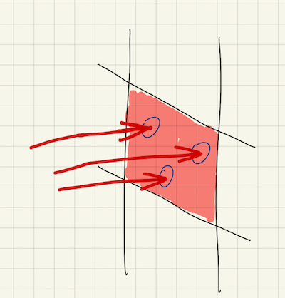
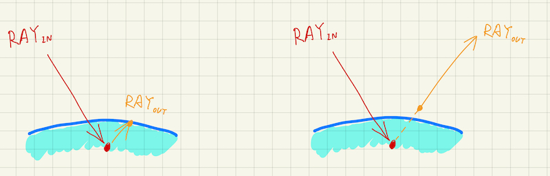
There is one detail here that deserves some explanation. Note how we compoute the new ray origin, ray_pos. We have shifted the hit position by a tiny offset along the new direction, i.e. eps * ray_dir. Without this shift, because of the numerical precision errors, sometimes the new ray would immediately intersect with the surface it has just hit, the so called self-intersection. This could result in very noisy artifacts where the objects are covered with small black dots. Here is an example to illustrate that artifact.
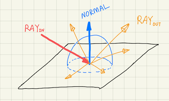
How to define sample_ray_dir()? We’ve briefly explained that a new ray direction should be picked randomly above the hit surface. (Again, this claim is only correct only for lambertian. In the later posts we will add specular and transmissive materials, where the new ray direction cannot be chosen arbitrarily.) One strategy for doing this is to choose a random point within a unit sphere that is centered at \(\boldsymbol{p} + \boldsymbol{n}\), where \(\boldsymbol{p}\) is the hit point and \(\boldsymbol{n}\) is the unit surface normal.
Let’s start with choosing a random point within a unit sphere centered at the origin \(\boldsymbol{\emptyset}\).
@ti.func
def random_in_unit_sphere():
    p = ti.Vector([0.0, 0.0, 0.0])
    while True:
        for i in ti.static(range(3)):
            p[i] = ti.random() * 2 - 1.0
        if p.dot(p) <= 1.0:
            break
    return p
What this function does is to keep proposing a 3-D point inside a [-1.0, +1.0] cube randomly, and terminates when the distance between the point and the zero origin is less than or equal to 1.0.
You may be wondering what ti.static is all about. Well, it tells Taichi to unroll your loop at compile time. This is a neat trick to gain performance without code duplication.
With this helper, we can easily write out how to sample a new direction:
@ti.func
def sample_ray_dir(indir, normal, hit_pos):
    return ti.normalized(random_in_unit_sphere() + normal)
In its most canonical form, this should have been:
hit_pos + ti.normalized(random_in_unit_sphere() + normal) - hit_pos
But then hit_pos gets canceled out. Albeit none of the args except for normal are used, we still pass them in, as they will be in the future posts.
Here’s the complete snippet for the ray tracing procedure:
@ti.func
def random_in_unit_sphere():
    p = ti.Vector([0.0, 0.0, 0.0])
    while True:
        for i in ti.static(range(3)):
            p[i] = ti.random() * 2 - 1.0
        if p.dot(p) <= 1.0:
            break
    return p

@ti.func
def sample_ray_dir(indir, normal, hit_pos, mat):
    return ti.normalized(random_in_unit_sphere() + normal)

@ti.kernel
def render():
    for u, v in color_buffer:
        ray_pos = camera_pos
        ray_dir = ti.Vector([
            (2 * fov * (u + ti.random()) / res[1] - fov * aspect_ratio),
            (2 * fov * (v + ti.random()) / res[1] - fov),
            -1.0,
        ])
        ray_dir = ti.normalized(ray_dir)

        px_color = ti.Vector([0.0, 0.0, 0.0])
        throughput = ti.Vector([1.0, 1.0, 1.0])
        depth = 0

        while depth < max_ray_depth:
            closest, hit_normal, hit_color, mat = intersect_scene(ray_pos, ray_dir)
            if mat == mat_none:
                break
            if mat == mat_light:
                px_color = throughput * light_color
                break
            hit_pos = ray_pos + closest * ray_dir
            depth += 1
            ray_dir = sample_ray_dir(ray_dir, hit_normal, hit_pos, mat)
            ray_pos = hit_pos + eps * ray_dir
            throughput *= hit_color

        color_buffer[u, v] += px_color
Let’s give it a shot, python3 box.py:
“Whaaaa?”
Recall how the scene is set up so far. We have created five planes, all of which have a lambertian material. However, no light source has ever been defined! All the rays have bounced tirelessly for a while, then gone in vein.
Let’s quickly hack up a light source. I’m going to switch the material of the top plane from mat_lambertian to mat_light, a one line change.
@ti.func
def intersect_scene(ray_o, ray_d):
    # ...

    # top
    # ...
    # if 0 < cur_dist < closest:
        # ...
        color, mat = gray, mat_light  # mat_lambertian
If we run the example again:
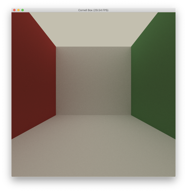
Voila! Our hard working has finally paid off.
I’d like to end the post here, because this should be enough for one with no CG experience to digest for a while. If you have followed this far, thank you for your time and patience! In the next post, I will be adding the rest of the components to the scene, including a rectangular light source, and two spheres with apparently different materials. For any problem you might encounter, here is my implementaion. If you are yearning for more, think about how to check for ray-rectangle and/or ray-sphere intersections, and try extending the example for yourself :)
Well, the original implementation in this series was in fact forked from Yuanming’s wonderful
sdf_renderer.py, but there are only these many ways to write a ray tracer, and they all look alike. Who is Yuanming? The Father of Taichi! ↩This is only true on GPU, since on CPU, the number of threads we can launch is usually much less than the size of the tensor. On the other hand, CPU cores are much more powerful and can finish the computation per coordinate much faster. ↩